TidyTuesday: Pixar Film Ratings

Which Pixar Films have the best and worst ratings? We answer that question with a dumbbell plot made from this week’s TidyTuesday data. To create this plot, first we download the data from GitHub. There are two tables, one table has information about the films (run time, release date, etc.) and the other table has information about the films ratings from sources like Rotten Tomatoes and Metacritic.

# Download data
import pandas as pd

base_url = "https://raw.githubusercontent.com/rfordatascience/tidytuesday/main/data/2025/2025-03-11"
films = pd.read_csv(f"{base_url}/pixar_films.csv")
response = pd.read_csv(f"{base_url}/public_response.csv")

Let’s clean the data by dropping columns and rows that we don’t use, computing the mean film rating, and sorting the records by mean rating. I didn’t end up using data from the films table for the plot, but it is still interesting to look at the release date and run time of the films so I kept the join step.

# Wrangle data to get in proper format for table and plotting
df = (
    films.merge(response, on="film")
    .drop(columns=["critics_choice", "number", "cinema_score", "film_rating"])
    .dropna(subset=["rotten_tomatoes", "metacritic"], how="all")
    .assign(
        mean_rating=lambda x: x[["rotten_tomatoes", "metacritic"]].mean(axis=1),
        run_time=lambda x: x["run_time"].astype(int),
        release_date=lambda x: pd.to_datetime(x["release_date"]).dt.strftime(
            "%b %d, %Y"
        ),
    )
    .sort_values("mean_rating", ascending=True)
    .reset_index(drop=True)
)

Let’s look at the data in a table.

# Display data in a table
from IPython.display import HTML

# Clean up column titles, reverse row order, and convert to HTML
df2 = df.copy()
df2.columns = df2.columns.str.replace("_", " ").str.title()
html_table = df2.iloc[::-1].to_html(index=False)

display(HTML(html_table))

Film	Release Date	Run Time	Rotten Tomatoes	Metacritic	Mean Rating
Toy Story	Nov 22, 1995	81	100.0	95.0	97.5
Ratatouille	Jun 29, 2007	111	96.0	96.0	96.0
Inside Out	Jun 19, 2015	95	98.0	94.0	96.0
Toy Story 3	Jun 18, 2010	103	98.0	92.0	95.0
WALL-E	Jun 27, 2008	98	95.0	95.0	95.0
Finding Nemo	May 30, 2003	100	99.0	90.0	94.5
Toy Story 2	Nov 24, 1999	92	100.0	88.0	94.0
The Incredibles	Nov 05, 2004	115	97.0	90.0	93.5
Up	May 29, 2009	96	98.0	88.0	93.0
Toy Story 4	Jun 21, 2019	100	97.0	84.0	90.5
Soul	Dec 25, 2020	100	96.0	83.0	89.5
Coco	Nov 22, 2017	105	97.0	81.0	89.0
Monsters, Inc.	Nov 02, 2001	92	96.0	79.0	87.5
Incredibles 2	Jun 15, 2018	118	93.0	80.0	86.5
Finding Dory	Jun 17, 2016	97	94.0	77.0	85.5
A Bug's Life	Nov 25, 1998	95	92.0	77.0	84.5
Onward	Mar 06, 2020	102	88.0	61.0	74.5
Brave	Jun 22, 2012	93	78.0	69.0	73.5
Cars	Jun 09, 2006	117	74.0	73.0	73.5
Monsters University	Jun 21, 2013	104	80.0	65.0	72.5
The Good Dinosaur	Nov 25, 2015	93	76.0	66.0	71.0
Cars 3	Jun 16, 2017	102	69.0	59.0	64.0
Cars 2	Jun 24, 2011	106	40.0	57.0	48.5

Now we create the dumbbell plot, click the code button below to show the code.

# Create dumbbell plot of film ratings
import seaborn as sns
import matplotlib.pyplot as plt

# Set plot style
sns.set_style("whitegrid", {"grid.color": "lightgrey"})

# Create the dumbbell plot
plt.figure(figsize=(10, 9))
for _, row in df.iterrows():
    plt.plot(
        [row["rotten_tomatoes"], row["metacritic"]],
        [row["film"], row["film"]],
        color="black",
        linewidth=1,
        zorder=1,  # Keeps lines behind markers
    )
    plt.scatter(
        row["rotten_tomatoes"],
        row["film"],
        color="#CD0BBC",
        label="Rotten Tomatoes" if _ == 0 else "",
        s=100,
    )
    plt.scatter(
        row["metacritic"],
        row["film"],
        color="#61D04F",
        label="Metacritic" if _ == 0 else "",
        s=100,
    )
    plt.scatter(
        row["mean_rating"],
        row["film"],
        color="#2297E6",
        label="Mean Rating" if _ == 0 else "",
        s=100,
    )

# Add labels and title
plt.xlabel("Film Rating", fontsize=14)
plt.ylabel("")
plt.title(
    "Rotten Tomatoes Ranks Pixar Films Higher than Metacritic, Except for Cars 2",
    fontsize=16,
)
plt.xticks(fontsize=12)
plt.yticks(fontsize=12)
plt.legend(fontsize=14)

# Save the plot as an image for the blog listing
plt.savefig("image.png", dpi=300, bbox_inches="tight")

# Show the plot
plt.show()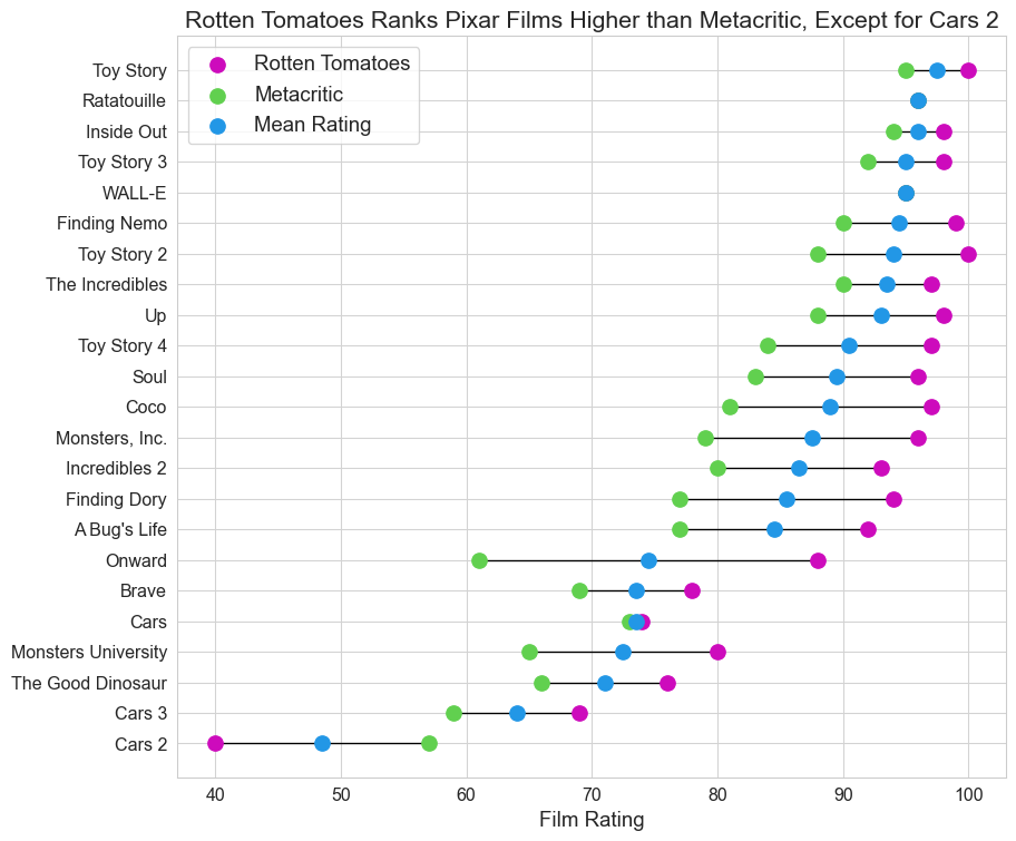

We see that Toy Story has the highest average rating and Cars 2 has the lowest average rating. Two films, Ratatouille and WALL-E, have the same rating on Rotten Tomatoes and Metacritic. Cars 2 is the only film that received a higher Metacritic rating than Rotten Tomatoes rating.