Average Area of a Random Triangle

This post shows how to compute the expected value of the area of a random triangle analytically, numerically, and with Monte Carlo. Specifically, suppose the vertices of a triangle are sampled uniformly from the perimeter of a circle with radius one (see picture). What is the expected value of the area of the triangle? Is it 0.5? Is it \(\pi\)/5? In this post, I’ll share how I solved this problem.

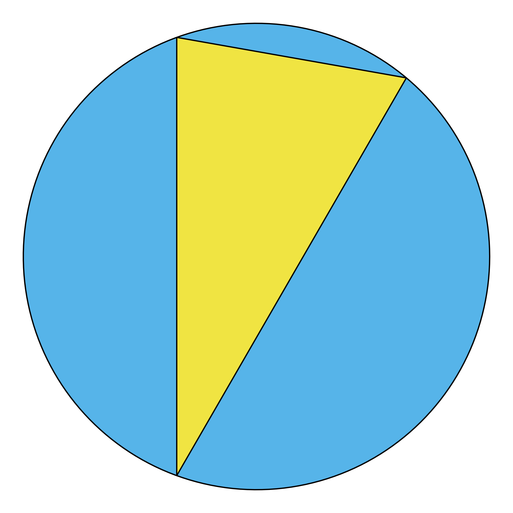
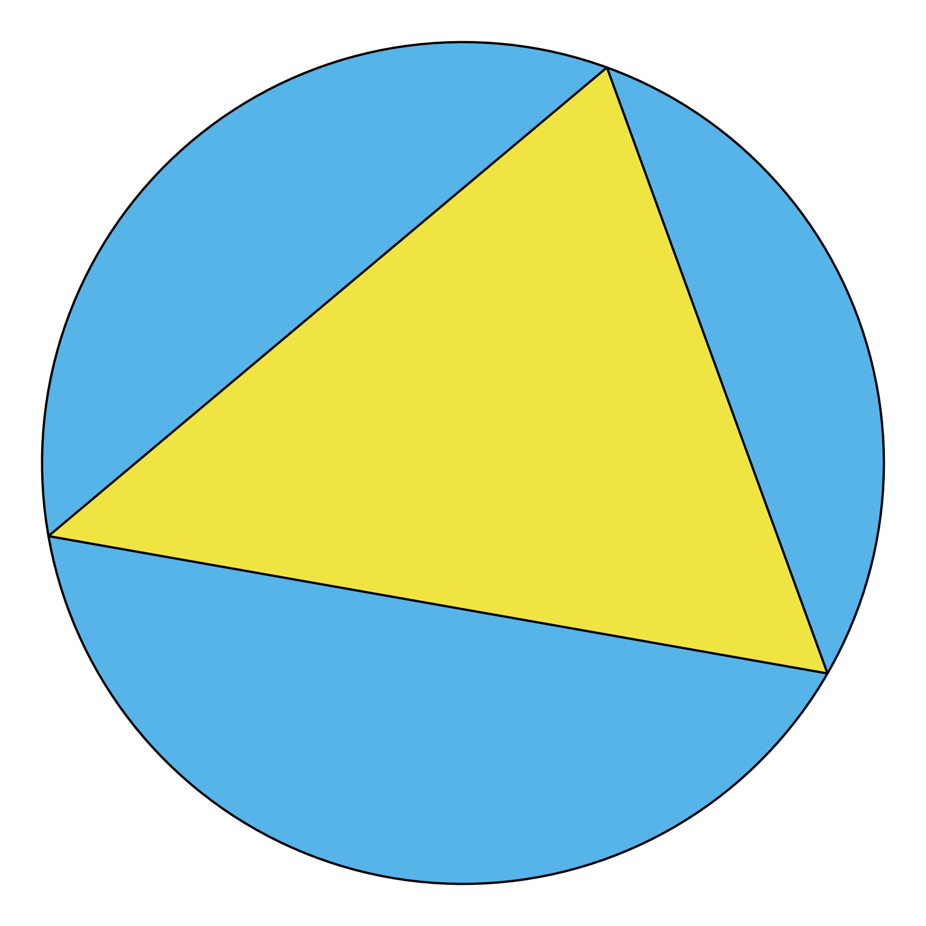
Figure 1: Two triangles inscribed in a circle. In our set-up, the blue circle has radius one and the vertices of the triangle are sampled uniformly on the perimeter of the circle. Our goal is to compute the average area of the triangle.

First, I tried to find a closed-form expression for the expected value of the area. I expressed the \(i\)th triangle vertex as \((X_i,Y_i)\), where \(X_i=\cos(\theta_i)\), \(Y_i=\sin(\theta_i)\), and \(\theta_i\sim \textrm{Unif}(0,2\pi)\) for \(i=1,2,3\). I then searched on Google for the area of the triangle, and found the formula \[ A=\frac{1}{2}|X_1(Y_2-Y_3)+X_2(Y_3-Y_1)+X_3(Y_1-Y_2)|, \] which is half of the absolute value of the determinant of a matrix whose columns are \((X_1,X_2,X_3)\), \((Y_1,Y_2,Y_3)\), and \((1,1,1)\). Now, this formula depends on three angles, so I asked myself whether we could make a simplifying assumption that would reduce the dimension of the problem to two. After some thought, I realized that we can rotate the triangle so that \(X_1=1\) and \(Y_1=0\), which effectively sets \(\theta_1=0\) and leaves the area unchanged since rotation matrices have determinant one. This simplifies the area formula to \[ A=\frac{1}{2}|Y_2-Y_3+X_2Y_3-X_3Y_2|. \] The term \(X_2Y_2-X_3Y_2\) looks like a trig identity, and so I searched on Google and found that \[ X_2Y_3-X_3Y_2=-\sin(\theta_2-\theta_3), \] allowing the area to be further simplified to \[ A=\frac{1}{2}|\sin(\theta_2)-\sin(\theta_3)-\sin(\theta_2-\theta_3)|. \] I didn’t see how to simplify this expression further, so I moved on to the expected value calculation.

Since the angles \(\theta_2\) and \(\theta_3\) have joint density \(1/(4\pi^2)\), the expected value of the area is \[ E[A]=\frac{1}{8\pi^2}\int_0^{2\pi}\int_0^{2\pi}|\sin(\theta_2)-\sin(\theta_3)-\sin(\theta_2-\theta_3)|\;d\theta_2\;d\theta_3. \] At this point I got stuck since I wasn’t sure how to deal with the absolute value in the integrand. 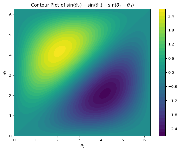Eventually I remembered that an absolute value can be written as a sum of a positive and a negative term, which applied to our problem leads to \[ E[A]=\frac{1}{8\pi^2}\left[\int\int_{f(\theta_2,\theta_3)>0}f(\theta_2,\theta_3)\;d\theta_2\;d\theta_3 - \int\int_{f(\theta_2,\theta_3)<0}f(\theta_2,\theta_3)\;d\theta_2\;d\theta_3 \right], \] where \[ f(\theta_2,\theta_3)=\sin(\theta_2)-\sin(\theta_3)-\sin(\theta_2-\theta_3). \] This looks a little better, and there’s a hint of symmetry so I plotted the function and realized that 1) the second integral in the square brackets is the negative of the first integral and 2) the region over which \(f(\theta_2,\theta_3)\) is positive is \(\theta_3>\theta_2\). Here is a plot of the \(f\) function, the code to generate the plot can be expanded by clicking on the arrow icon. Note that the axes limits are \((0,2\pi)\).

import numpy as np
import matplotlib.pyplot as plt


def f(theta2: float, theta3: float) -> float:
    return np.sin(theta2) - np.sin(theta3) - np.sin(theta2 - theta3)


# Create mesh grid
theta2 = np.linspace(0, 2 * np.pi, 100)
theta3 = np.linspace(0, 2 * np.pi, 100)
Theta2, Theta3 = np.meshgrid(theta2, theta3)
Z = f(Theta2, Theta3)

# Plot contour
plt.figure(figsize=(8, 6))
contour = plt.contourf(Theta2, Theta3, Z, levels=50, cmap="viridis")
plt.colorbar(contour)
plt.xlabel(r"$\theta_2$")
plt.ylabel(r"$\theta_3$")
plt.title(
    r"Contour Plot of $\sin(\theta_2) - \sin(\theta_3) - \sin(\theta_2 - \theta_3)$"
)
plt.show()

It follows that the formula for the expected value of the area can be simplified to \[ E[A]=\frac{1}{4\pi^2}\int_0^{2\pi}\int_{\theta_2}^{2\pi}f(\theta_2,\theta_3)\;d\theta_3\;d\theta_2. \] I computed this last expression using WolframAlpha and found that the double integral equals \(6\pi\), which implies \[ \boxed{E[A]=\frac{3}{2\pi}}. \] What a pleasant surprise!

While I was stuck on this integral, I computed the expected value numerically and with Monte Carlo. Here is the code:

import scipy.integrate as spi


def triangle_area(theta1: float, theta2: float) -> float:
    """Compute the area of a triangle inscribed in a unit circle and with
    vertices at 0, theta1, and theta2 radians.
    """
    X2 = np.cos(theta1)
    X3 = np.cos(theta2)
    Y2 = np.sin(theta1)
    Y3 = np.sin(theta2)
    area = 0.5 * np.abs(Y2 - Y3 + X2 * Y3 - X3 * Y2)
    return area


def compute_monte_carlo(n: int = 1_000_000, seed: int = 1) -> float:
    """Compute expected value of triangle area using Monte Carlo."""
    np.random.seed(seed)
    theta1, theta2 = np.random.uniform(low=0, high=2 * np.pi, size=(2, n))
    areas = triangle_area(theta1, theta2)
    return np.mean(areas)


def compute_numerical_integral() -> float:
    """Compute expected value of triangle area using numerical integration."""
    result, _ = spi.dblquad(triangle_area, 0, 2 * np.pi, 0, 2 * np.pi)
    result /= 4 * np.pi**2
    return result


# Compute expected value using both methods
integral_est = compute_numerical_integral()
mc_est = compute_monte_carlo()

Let’s put the results in a table to compare them.

import pandas as pd
from IPython.display import Markdown

data = {
    "Method": ["Exact Value", "Numerical Integration", "Monte Carlo"],
    "Expected Area": [3 / 2 / np.pi, integral_est, mc_est],
}
df = pd.DataFrame(data)

# Format numeric values to three significant figures
df = df.map(lambda x: f"{x:.4g}" if isinstance(x, float) else x)

markdown_table = df.to_markdown(index=False)

styled_table = f"""
<div style="display: inline-block; width: 40%; min-width: 200px;">
{markdown_table}
 </div>
"""

display(Markdown(styled_table))

Table 1: Comparison of values for the average area.

Method	Expected Area
Exact Value	0.4775
Numerical Integration	0.4775
Monte Carlo	0.4773

It’s great to see all three methods give the same answer. Overall, this was a fun exercise and gave me an excuse to get some experience creating a blog with Quarto!